In the previous post, we discussed that understanding time series analysis is a prerequisite for learning spatio-temporal modeling.

Time series data are:

Observations or measurements that are indexed according to time

There is an ordering to the time series data, so it is generally not independent. Imagine a simple non-temporal data such as heights $X_{i}$ and weights $Y_{i}$ of all students in a class. We can randomly permute the indices of the data. However, for time series data such as height and weight of a student $X_{t}$ and $Y_{t}$ from 1 to 20 years old, we cannot change the order of the data.

Time Scales

Depending on the temporal granularity of observations, time series data can be aggregated at different time scales such as yearly, monthly, daily, hourly, or even microseconds for stocks. The time series book gave an example about studying the effect of PM10 on deaths at a yearly or a daily basis, and stated that:

The daily average looks at short-term changes and could prehaps be interpreted as representing “acute” effects of pollution, while the yearly average might represet “chronic” effects of air pollution levels.

Fixed vs. Random Variation

The time series book states

that many real time series in the world are composed of what we might think of as fixed and random variation,, but many time series books tend to image a time series as consising only of random phenomena. For example,

One model is to model daily Baltimore temperature as a function flucuating around the mean temperature of all time span $\mu$. [ y_t = \mu +\epsilon_t\tag{1} ]

Another way is to model daily Baltimore temperature as a funciton of the previous data temperature. [ y_t = y_{t-1}+\epsilon_t\tag{2} ]

The model (1) uses fixed variation, and the model (2) uses random variation, as the former assumes that all errors flucuate around the mean, while the latter assumes the errors flucuate around the previous day temperature.

Note that: fixed vs. random variation are different from fixed and random effects in mulitlevel modeling. If the readers have the background of pyschology or experimental design, time series data can be easily understood as “repeated measures design” or “within-subject design”. It is sometimes called panel data. The data is collected through a series of repeated observations of the same subjects over some extended time frame.

A common approach to model panel data is to use linear mixed-effect model. In matrix notation: [ y = X\beta + Zu + \epsilon ] where $y$ is the $n \times 1$ vector of reponses, $X$ is an $n \times p$ design/covariate matrix for the fiexed effects $\beta$, and $Z$ is the $n \times q$ design/covariate matrix for the random effects $u$. The $n \times 1$ vector of errors $\epsilon$ is assumed to be the multivariate normal distribution with mean 0 and variation matrix $\sigma_{\epsilon}^2R$.

The difference between mixed/random variation and mixed effect model is that the latter deals with time series data of mulitple subjects. For example, if we model temperature of mulitple cities such as DC, NYC, and Baltimore, then we can use mulitlevel modeling.

The Goals of Time Series Analysis

The goals of time series analysis are almost the same as the goals of spatio-temporal analysis as we discussed here. I will use the description and examples from the time series book instead of math formula to illustrate the goals of time series.

1.Smoothing: given a complete (noisy) dataset, what can I infer about the true state of nature in the past?

• Given a noisily measured signal, can I reconstruct the true signal from the data?
• Now that my spacecraft has flown around the moon, what the distance of its closest approach to the moon?

2.Filtering: given the past and the present observation, how should I update my estimate of the true state of nature?

• Given my current estimate of my spacecraft’s position and velocity, how should I update my estimate of position and velocity based on new gyroscope and radar measurements?
• Given the history of monthly unemployment data in the U.S. and my estimate of the current unemployment level, how should I revised my estimate based on the Bureau of Labor Statistics’ latest data release?
• Given the history of endowment returns, the current year return, and the need for spending a target percentage of the endowment value every year, how much should a University spend from the endowment in the following fiscal year?

‘true state of nature’ stands for the hidden state in HMM introduced in the previous post.

3.Forecasting: given the past and the present, what will the future look like (and its uncertainty)?

• Given the past 10 years of quarterly earnings per share, what will next quarter’s earnings per share be for Apple, Inc.?
• Given global average temperatures for the past 200 years, what will global average temperatures be in the next 100 years?

4.Time Scale Analysis: given an observed set of data, what time scales of variation dominate or account for the majority of temporal variation in the data.

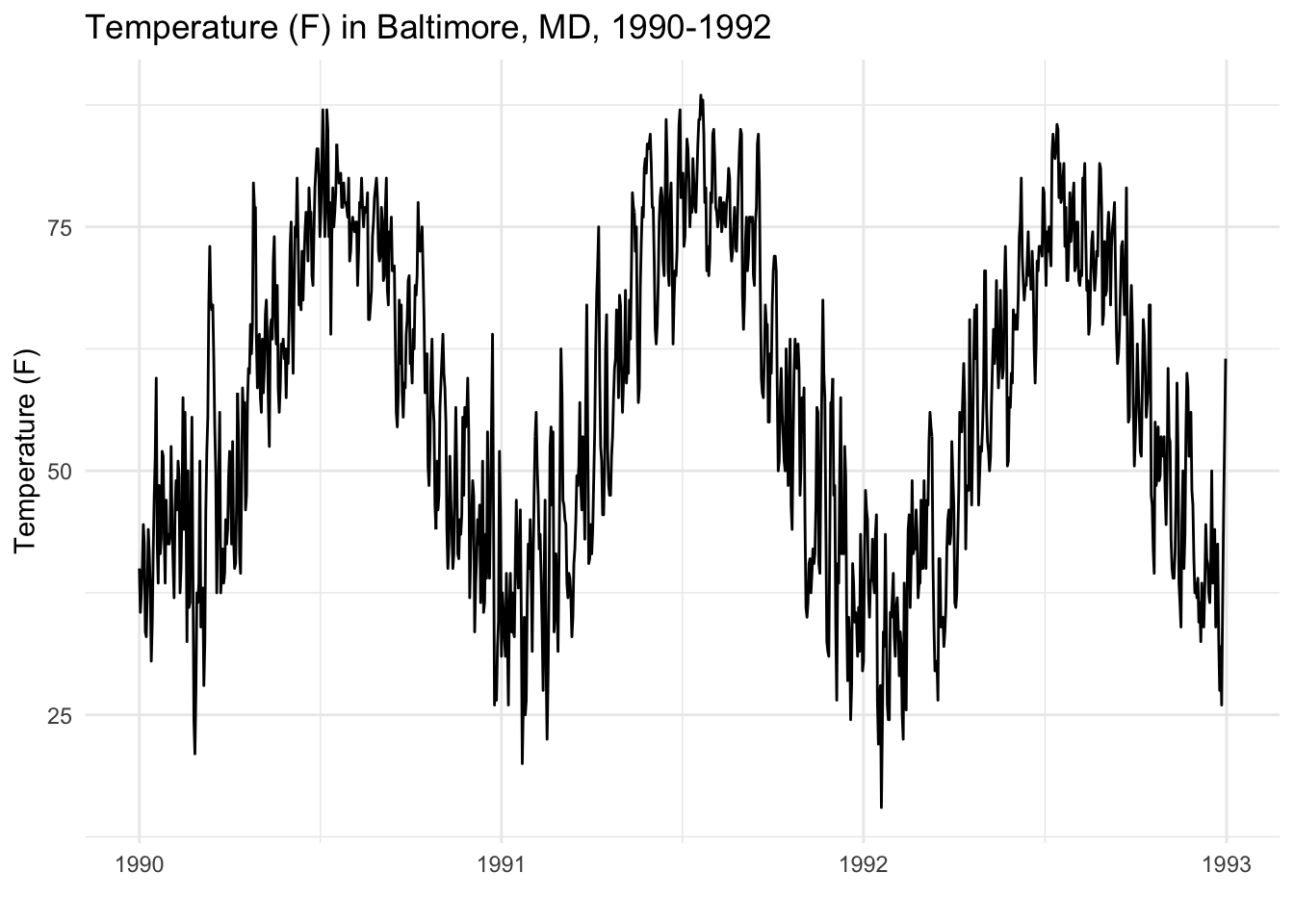
• Is there a strong seasonal cycle in the observations of temperature in Baltimore, MD?
• Is the association between ambient air pollution and mortality primarily driven by large annual changes in pollution levels or by short-term spikes?

5.Regression Modeling: given a time series of two phenomena, what is the association between them?

• What is the association between daily levels of air pollution and daily values of cardiac hospitalizations?
• What is the lag (in months) between a change in a country’s unemployment rate and a change in the gross domestic product?
• What is the cumulative number of excess deaths that occurs in the 2 weeks following a major hurricane?

Examples

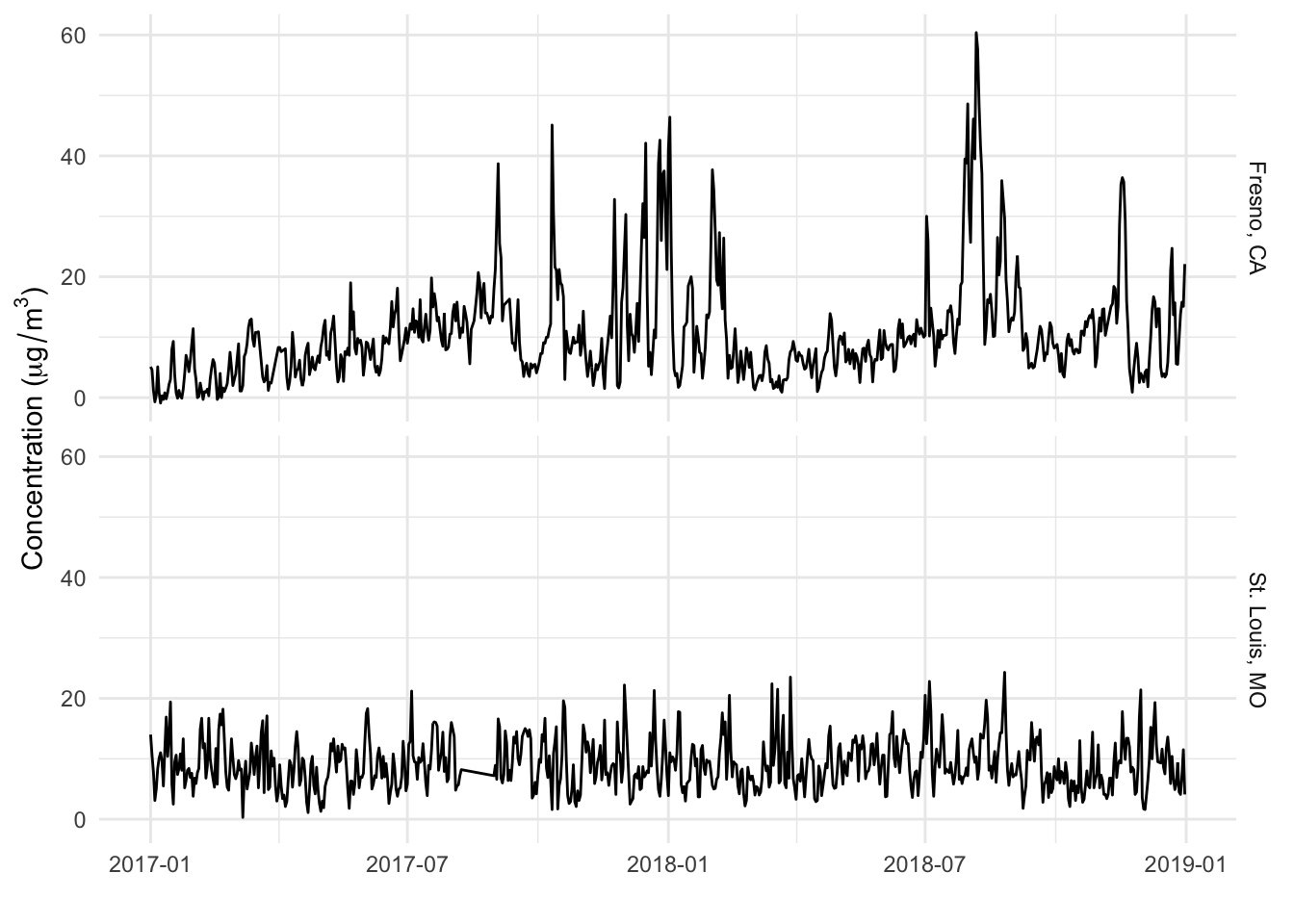
The timeseriesbook used the air pollution data of two cities to illustrate time series analysis.

Four critical components to understanding the structure of many kinds of time series are:

• Linear trends (increasing and decreasing) over time
• Seasonality, yearly periods over time
• Overall level (mean) across time
• Variability (spikiness) across time

Trend-Season-Residual decomposition is to examine the trend, season, and residuals for a time series. It is the beginning of time scale analysis in many time series analyses.

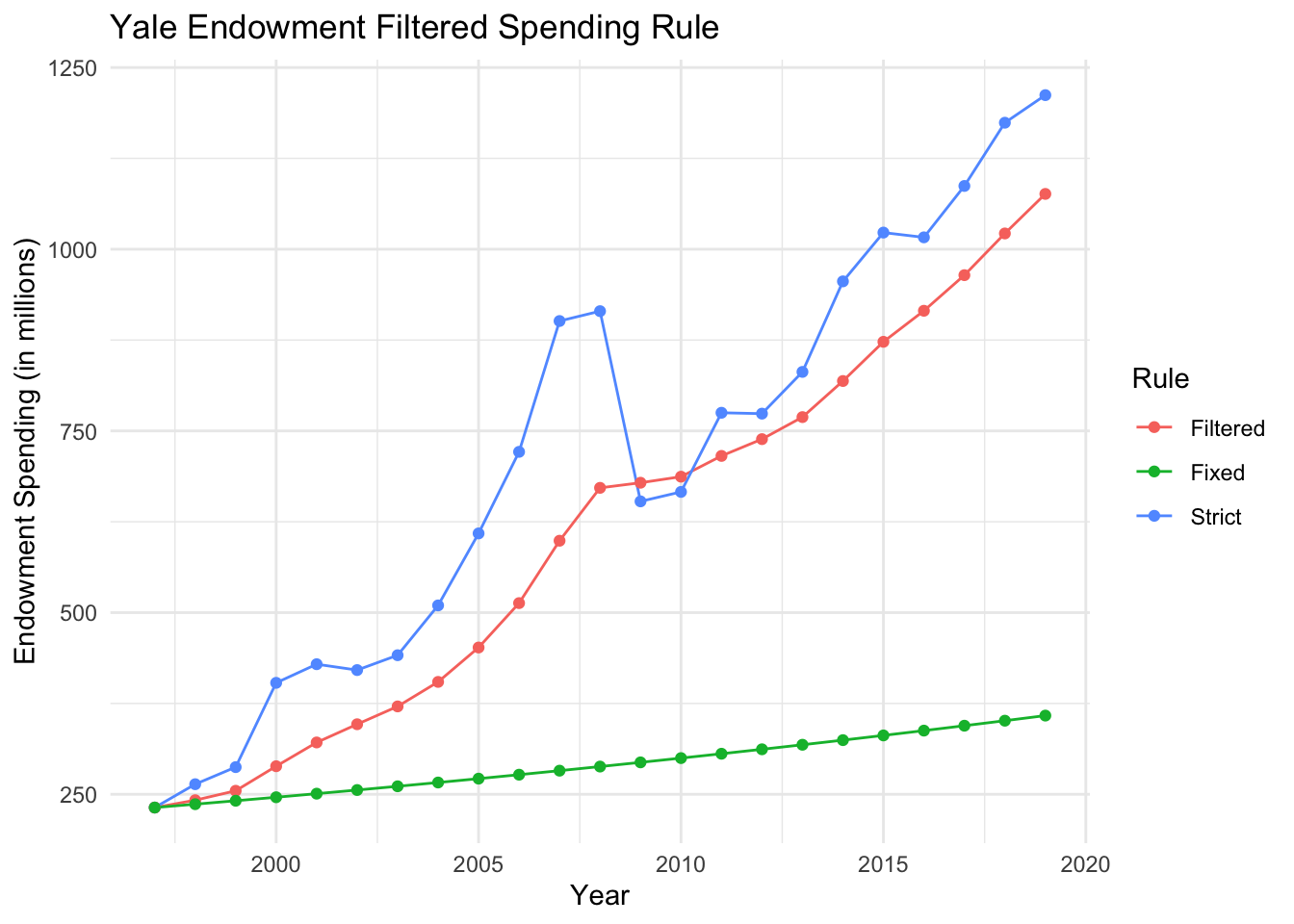
The timeseriesbook then provided another example of Yale endowment spending to illustrate the basic idea of Karman filter.

.

The plot above shows the spending patterns based on a stricted 4% spending rule (“Strict”), a fixed spending rule indexed to inflation (“Fixed”), and a filtered spending rule using the complementary filter with λ = 0.8 (“Filtered”). Clearly, the filtered rule underspends relative to the endowment’s annual market value, but tracks it closer than the fixed rule and smooths out much of the variation in the market value.

Stationarity

The timeseriesbook then introduced an important concept of stationarity for time series data. Actually, stationarity is a critical concept in spatio-temporal modeling. Understanding temporal stationarity will help us better understand spatial stationarity later on.

Strictly stationary mean that, for a time series $X_1, X_t, \dots$ :

if any subset of the time series, $(Y_{t_1},Y_{t_2},Y_{t_n})$, with size n and any integer $\tau$, it has the same joint distribution as $(Y_{t_1+\tau},Y_{t_2+\tau},Y_{t_n\tau})$.

Some may wonder why we define strictly stationary in this way. Why not simply define that for all $t$, the mean and variance of the subset ${Y_t}$ is constant. The simple answer is that the subset $Y_t$ is just a special situation that $n = 1$. However, strictly stationary requires more for future modeling: for any size n of the subset, the joint distribution of this subset is the same with all shifts’ joint distribution. Note that, it does not require the distributions to be the same for all permutation of the same size subsets, as time series data is an ordering data. In other words, a stationary time series is invariant to shifts.

The most basic assumption for a data $X_1, \dots,X_n$ is that $X_i$ is independent, as a lot of nice results hold for independent random variables such as law of large numbers and central limit theorem. However, as we all know that time series are usually not independent. There are many ways of dependence, and stationarity is just one type of dependence structure. The good thing is those nice results such as central limit theorem still hold for stationary time series. Therefore, if the time series have stationarity, we can use ARMA(AutoRegressive Moving Average) to model it. For non-stationary data, after certain transformation such as differencing, we can assume the data becomes stationary. This model process is so-called ARIMA(AutoRegressive Integrated Moving Average).

Strictly stationary is difficult to require, so we usually use a weaker concept: Second-order stationary: if the mean is constant and the covariance between any two values only depends on the time difference between those two values.

\begin{align} E[Y_t] &= m \\ Cov(Y_t,Y_{t+\tau}) &= \gamma(\tau) \end{align}

In a strictly stationary time series, the moments of all orders remain constant throught time. However, second order stationarity only requires that first and second order moments (mean, variance and covariances) are constant throughout time.

The basic idea of stationarity is that the distribution of the time series data does not depend on t. How to understand that? Well, image that at a given time t, the value of the time series data is determined by a statistical distribution… let’s say normal distribution.. the data at different time t are not independent, but we assume that (1) all data are generated based on the same model (i.e., the distribution parameters such as mean and variance are the same) and (2) the data are correlated in a way that the closer the time lag is, the larger or the smaller (or whatever relation the covariance is. No matter how the covariance changes, it changes as a funtion of time difference (or time lag) instead of the time t itself.

Note that:

In traditional regression settings we might assume that the residual variation is independent and identically distributed (iid), but in the time series context, there might be some residual autocorrelation remaining, even if the series is stationary.

Autocorrelation

One summary statistic of a stationary time series is the auto-correlation function (aka ACF). This is simply the auto-covariance function $\gamma(\tau)$ divided by $\gamma(0)$, which is the data variance. [ ACF(\tau) = { \gamma(\tau) \over \gamma(0) } ] As a result, the ACF(0) is always 1 and usually we plot that even thought it’s the same every time. We also assume that when $\tau \to \infty$, $\gamma(\tau) \to 0$, so for distance/time between points too far away do not affect each other (i.e., they are independent).

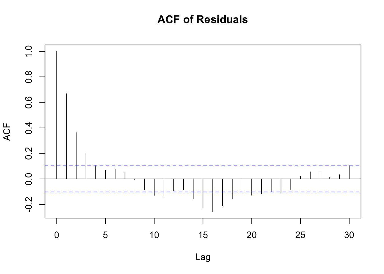
As mentioned above, in the time series context, there might be some residual autocorrelation remaining, even if the series is stationary. The timeseriesbook showed the ACF plot of the residuals from the Baltimore temperature data, after removing a monthly mean.

The ACF plot clearly shows there is some short-term auto-correlation left in the residuals. What to do about this will depend on the application and question at hand and we will discuss this further in the section on time series regression modeling.

Gaussian Processes

The definition of Gaussian process in wikipidia is:

a Gaussian process is a stochastic process (a collection of random variables indexed by time or space), such that every finite collection of those random variables has a multivariate normal distribution.

In the time series context, we can understand Gaussian process as a special stationary process whose joint distribution is Gaussian. For more details, seehere. The most important operation for Gaussian Processes (GP) is conditioning, as it allows Bayesian inference. In the case of Gaussian processes, Bayesian inference is to update the current hypothesis as new information (i.e., training data) becomes available. Thus, we are interested in the conditional probability $P_{X|Y}$.

The covariance matrix is determined by its covariance function, which if often called the kernel of the Gaussian process. We just mentioned that for stationary time series data (or second-order stationary), covariance between two random variables at different times only changes as a function of the time difference (lag).

Correspondingly, the Kernels of GP can also be separated into stationary and non-stationary kernels. Stationary kernels, such as the RBF kernel or the periodic kernel, are functions invariant to translations. That is, the covariance of two points (two random variables at two different time) is only dependent on their relative position.